Explaining the squarified treemap algorithm
As part of the visualization support, Glamorous Toolkit offers an implementation of a squarified Treemap. The algorithm is responsible for creating visualizations such as this one:
The implementation is captured in GtGraphTreemapSquarify
and a few adjacent helper classes. But how does it work?
One way to answer the question is to read the code. However, this particular algorithm was already published in Squarified Treemaps, Bruls et al., 2000, a paper that starts with the following abstract:
"An extension to the treemap method for the visualization of hierarchical information, such as directory structures and organization structures, is presented. The standard treemap method often gives thin, elongated rectangles. As a result, rectangles are difficult to compare and to select. A new method is presented to generate layouts in which the rectangles approximate squares."
The paper details the algorithm in several ways, but the core of the explanation is based on this depiction showing the steps that the algorithm takes for a specific input.
The example in the picture is about laying out nodes with the following weights #(6 6 4 3 2 2 1). The whole idea of the algorithm is to choose subdivisions that preserve the desired ratio. The diagram shows both the accepted and the rejected choices.
This picture is worth a thousand words. Of course, the primary intent of implementing an algorithm is to get to the final result. But our goal is not only to produce a functional system. We want an explainable system. The rule of thumb is that if a human deems a representation as meaningful, it should be the responsibility of the system to carry it forward.
So, naturally, we want our implementation to offer this kind of view, too.
In our case, when we inspect an instance of GtGraphTreemapSquarify
, we see the picture showing the steps as in the paper! This picture is available as a contextual view (see the Steps Figure view below):
Once the algorithm object knows how to present itself, we document the code through examples that give us interesting algorithm objects. For example, take a look at GtGraphTreemapLayoutExamples>>#squarifyWithSevenNodes
.
And once we have examples, we can quickly write narratives. Just like this one!
At the start, the algorithm splits the initial rectangle. It chooses a horizontal subdivision because the rectangle is wider than it is tall. It then fills the left half with a single rectangle. The aspect ratio of this first rectangle is 2.67.
Next, it adds a second rectangle above the first. The worst aspect ratio improves to 1.5.

However, if it adds the next area of size 4 above these original rectangles, then the aspect ratio of this rectangle degrades to 4.0.
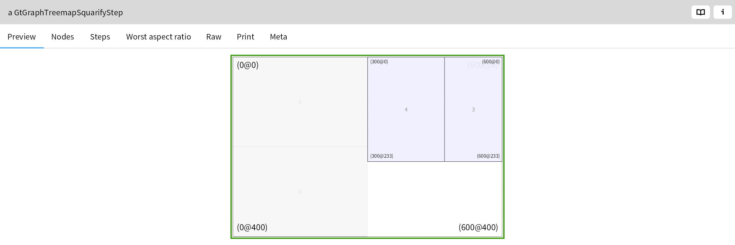
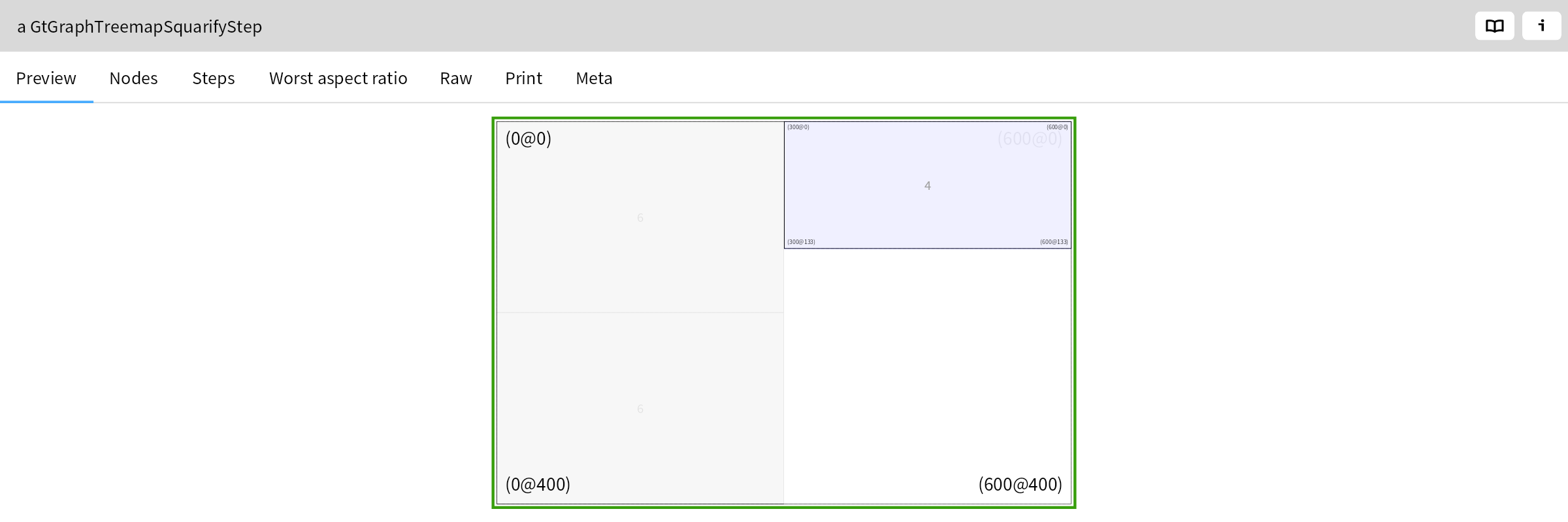
The algorithm therefore decides that it has reached an optimum for the left half in step two, and starts processing the right half. The initial subdivision it chooses here is vertical, because the rectangle is taller than it is wider. In step 4, it adds the rectangle with area 4:
In the next step, it adds area 3. The worst aspect ratio decreases from 2.25 to 1.81:
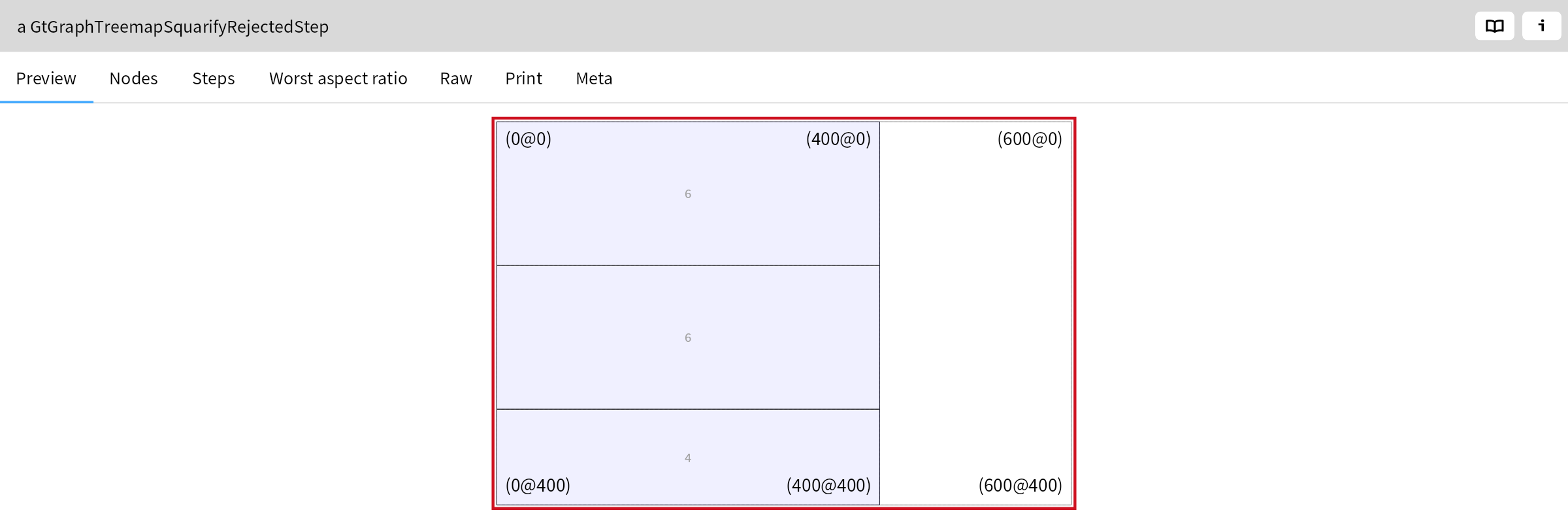
The addition of the next area (2), however, does not improve the result, as the worst aspect ratio increases from 1.81 to 4.5:
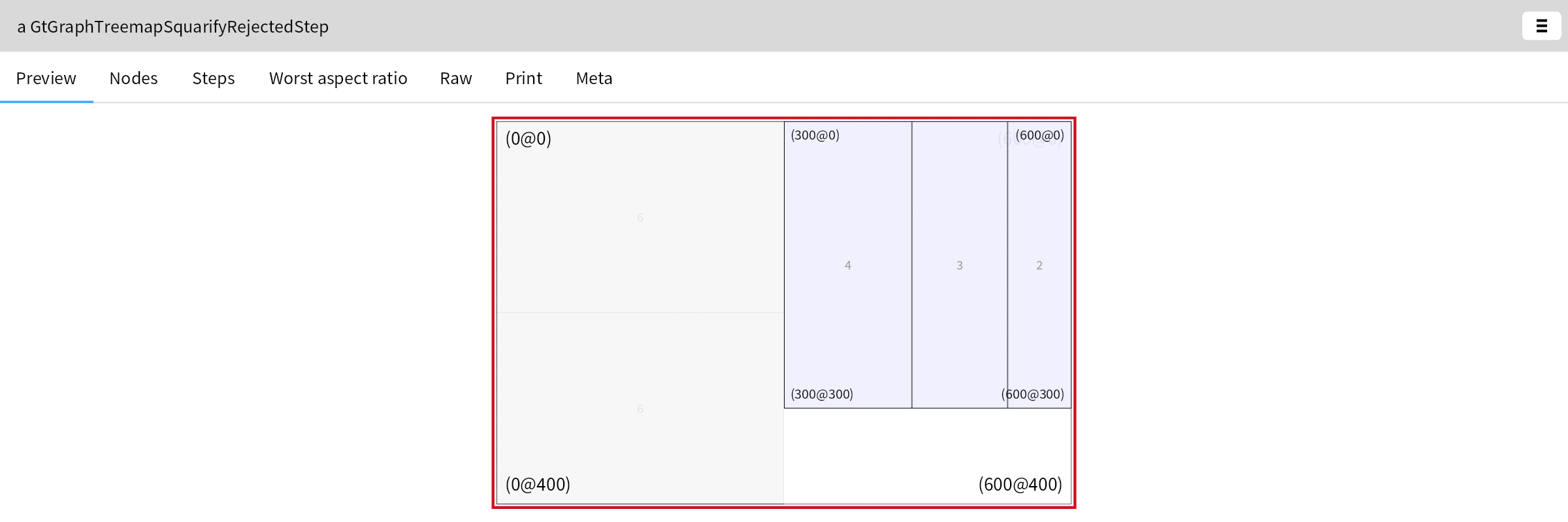
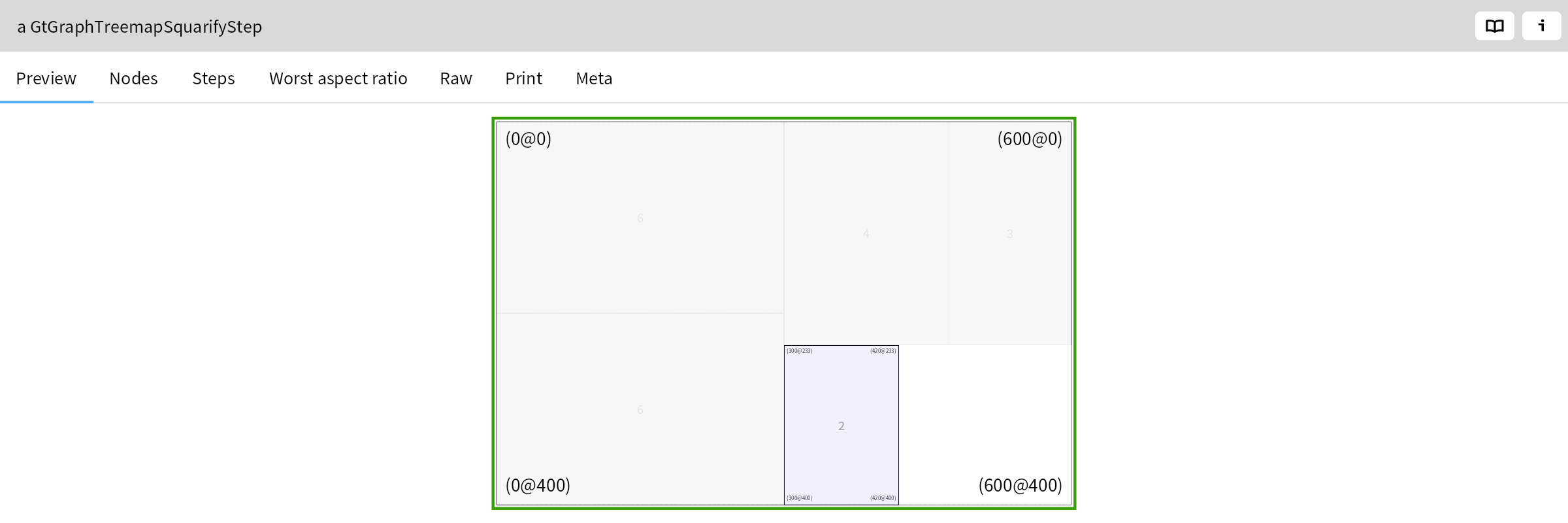
So it rejects this step and starts to fill the bottom right partition:

These steps are repeated until all rectangles have been processed. The final result is the following:
An optimal result cannot be guaranteed, and counterexamples can be constructed. The order in which the rectangles are processed is important. We found that a decreasing order usually yields the best results. The initially large rectangle is then filled first with the larger subrectangles.